
Financial markets do not merely facilitate the efficient exchange of capital — they provide the inspiration for passionate dinner table discussions, heated business meetings, and fierce social media debates across the globe. From Amazon’s latest strategic initiative to the trajectory of Bitcoin, having an opinion on major economic and industrial trends has been widely considered an essential characteristic of the sophisticated American for decades. This article does not seek to undermine the importance of or the passion many of us share for these topics, but rather to evaluate the prudence of paying someone else to decipher them. More specifically, it seeks to contrast the value proposition of what is commonly referred to as “active” portfolio management with that of comprehensive investment planning.
Willlam Sharpe, Nobel Laureate and Professor of Finance, Emeritus at Stanford University, offered a simplistic and satirical critique of paying someone to select superior investments in a 1991 Financial Analysts Journal article titled, The Arithmetic of Active Management1. He argues that in order to conclude that active stock selection will always underperform a more passive approach on average, one only needs to understand “the laws of addition, subtraction, multiplication and division”. Given that the collective return achieved by the total market must be comprised of the results of both passive investors (those who simply buy and hold the underlying stocks in proportion to their current market share) and active managers (those who attempt to outperform the market by overweighting certain stocks and underweighting others), and that a passive investor’s return will always equal that of the index, it follows that before costs are taken into consideration the return on the average actively managed dollar must be equal to that of the average passively managed dollar. Otherwise, the weighted average returns of the stocks purchased would somehow outperform the market itself. To illustrate, assume that the S&P 2 is composed of NFL and NBA — two newly issued stocks with respective market values of $1.5 trillion. On January 1, 2022, Speculative Financial completes its equity research and concludes that NFL is severely underpriced. As such, they use all of their capital to purchase $1 trillion of its common stock. Wheel of Fortune LLC sees things differently and chooses to allocate their trillion dollar portfolio exclusively to NBA. Instead of spending hours trying to identify the superior stock in advance, Sharpe Investing Inc. simply purchases $1 trillion of the S&P 2 Index Fund to efficiently gain equal exposure to both assets.
Further assume that in 2022, NFL issues a 12% dividend, while NBA returns only 2%. The equally-weighted S&P 2 and, by extension, the average dollar invested by Sharpe, earned 7% — the same return achieved by Speculative and Wheel of Fortune collectively. For the average active dollar to have outperformed, either NFL or NBA would have needed to yield more without a commensurate increase in the performance of the index — which is of course mathematically impossible. Furthermore, once the 1% management fee charged by both active firms to fund their respective research efforts is taken into account, the investment advisor industry actually underperformed. While this case describes a theoretical market with only two assets to choose from, trying to win with a fully-diversified portfolio often involves substantial transaction and tax costs as well as additional layers of management fees — making active management a true negative-sum game. So the next time someone tells you something along the lines of “In small stocks, especially, you’re probably better off with an active manager than buying the market”, you can kindly suggest that they would be better off with a review of elementary school arithmetic. While the distribution of manager performance may be wider in certain markets or during certain periods, the mean must always fall short.
The collective futility of traditional investment advice is not merely a sound academic theorem. It is an empirically proven reality. In an August 2000 edition of The Journal of Finance2, Professor Russ Wermers of the University of Maryland decomposed the combined performance of every U.S. stock fund from 1975 through 1994 into four components: Gross Performance — the return generated over and above that of the S&P 500 via superior stock picks, Management Fee — the average fund expense ratio, Not Fully Invested — the opportunity cost of holding cash to maintain fund liquidity, and lastly Transaction Costs — the expenses associated with making trades such as brokerage commissions (now mostly obsolete) and bid-ask spreads. While the average fund manager was able to achieve gross outperformance of 1.5% annually, the associated management fees of 1.1%, cash drag of .7%, and transaction costs of .5%, combined to drive down their net performance to -.8% relative to the index. Economist and author Burton Malkiel noted similar results in a 2005 study published by The Financial Review3, which found that during both the 10 and 20-year periods ending in 2003, 86% of the mutual funds that traded large-cap stocks underperformed the S&P 500.
Of course, demonstrating that a strategy merely fails on average is not enough to reject its viability. While it may be clear that the typical investment advisor is not worthy of your business, presumably a client with above average intelligence would have the capacity to identify an extraordinary performer such as Speculative Financial in advance. As we will soon see however, this idea is not supported by research nor is it particularly rational.
Consider the historical performance of John Hancock Fundamental All Cap Core I (JFCIX), a mutual fund that invests in companies with more than $10 billion in market value. From 2017 through 2021, JFCIX returned 146% while the S&P 500 yielded “only” 131%. On the surface, its managers Emory Sanders and Jonathan White look like very savvy investors. After all, their annualized return of 19.76% exceeded that of the benchmark by about 1.5 percentage points. A more thorough analysis, however, suggests that this was at best a mediocre performance.
The Capital Asset Pricing Model (CAPM), a Nobel Prize-winning framework for understanding financial markets, states that there is a positive linear relationship between an investment’s systematic risk — or the extent to which its price tends to respond to changes in the broader market — and the return investors demand from it. Thus, by running a linear regression of historical market returns on those of a specific portfolio, one can not only determine the latter’s relative volatility — or beta — but the return it was destined to generate in exchange.
The scatterplot below depicts the historical relationship between the weekly fluctuations of JFCIX and those of the index over the past five years. Each point represents the respective return of each entity during a particular week, with the x-axis value denoting the performance of the index, and the y-axis figure reflecting that of JFCIX.
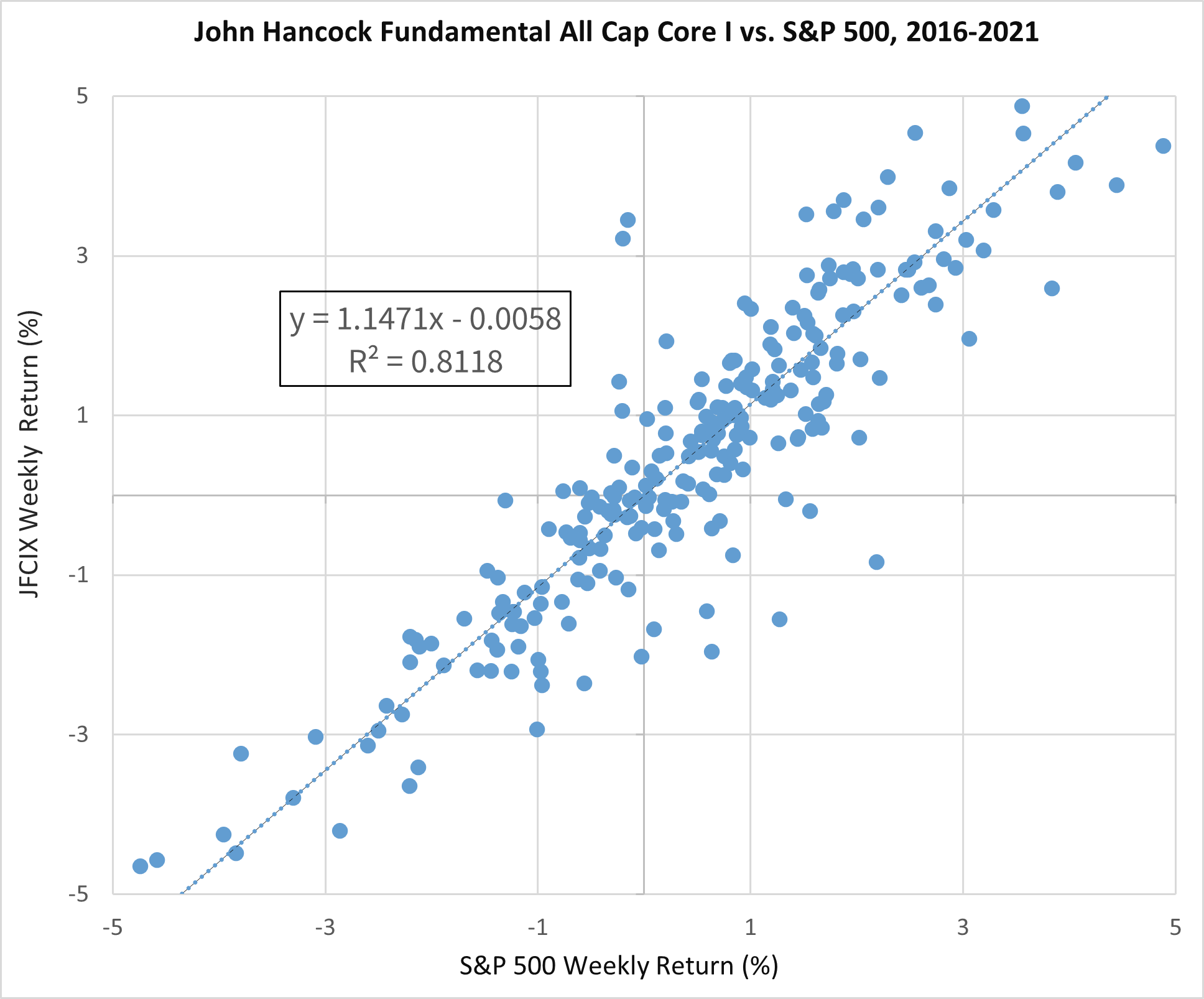
Not only is the correlation between these variables positive, but more importantly it is very distinct. Statistically speaking, this regression has an R-squared of .81, meaning that 81% of the weekly movement in JFCIX was influenced by developments in the broader large-cap market. If only 19% of its performance can be explained by factors unique to its underlying companies, we can take the slope of this regression seriously and start to draw some conclusions about the level of risk that Sanders and White have been taking. Specifically, we can state that this fund has a beta of 1.15 — or that for every 1% change in the value of the index, JFCIX fluctuates by 1.15%.
The CAPM suggests that this beta figure not only captures the relative volatility of JFCIX, but can also explain its outperformance. Specifically, it states that the expected return, or E(r) of an investment over a particular period is a function of:
R(f) + (β x [R(m) – R(f)])
Where:
R(f): The expected yield on a risk-free asset, such as the 10-year Treasury bill
β: The relative interim volatility of the asset, or beta
R(m): The expected return of the overall market, such as the relevant index
The primary idea behind the model is that investors are risk averse, given both the emotional and practical ramifications of portfolio volatility. While risks that are unique to an individual company can be easily mitigated by gaining exposure to the stock of a competitor, managing risks that impact the broader market such as a global pandemic is a far taller task. As such, the more sensitive a company’s cash flows are to such macroeconomic shocks, the higher the rate of return investors require of its stock in exchange. Only by comparing this built-in yield to its actual performance can we determine its true excess return, or alpha.
Inputting the relevant figures from our case study into the CAPM, the built-in annual return of JFCIX was:
1.08 + (1.15 x [18.27 – 1.08]) = 20.85
Given the 1.08% annual yield on the 10-year Treasury bill, the beta of 1.15 from our regression model, and the 18.27% annual return of the S&P 500, its managers were essentially handed a 20.85% return in exchange for the elevated volatility of the stocks they purchased. Thus, their 19.76% annual output actually underperformed the benchmark by 1.09% on a risk-adjusted basis.
To make matters worse for these investors, even a positive alpha measure would not have proven anything about their abilities.
Statistics 101 teaches that the more variable a series of observed outcomes, the greater the sample size needed to draw conclusions about its significance. The average percentage of a given number of daily free throw attempts made by a basketball player would be a far better indicator of underlying skill than the mean daily batting average achieved by a baseball player during the same number of at-bats. Due to the variability of the opposing pitching and other factors, the hitter’s daily output would be far more volatile and, in turn, provide less predictive value. The question is, how strong of a performance would Sanders and White have needed to prove that they weren’t just the beneficiaries of a few lucky economic or legislative bounces?
The most appropriate tool for this kind of statistical analysis is the One-Sample t-Test. By dividing the difference between an observed mean and a hypothesized mean by the standard error — a measure that penalizes smaller and more variable data sets — this model quantifies the significance of a given sample and, in turn, the probability that the hypothesized mean is wrong. More specifically, it yields an output known as a test statistic which depicts where a sample fell within the distribution of possible outcomes that could have taken place assuming the hypothesized mean is correct. Given that specified percentages of these outcomes tend to occur within various test statistic intervals, we can use sample performance data to ascertain the likelihood that a manager is more than just ordinary.
Assume that JFCIX returned 25.85% annually — an improvement of more than 6% over their actual output. While it may seem reasonable to utilize the resulting 5% annualized alpha measure as the observed mean of this sample, a closer look suggests that a different definition of average will be necessary.
Interestingly, the return that an investment earns over the course of several years (annualized return) is rarely the same as its average return. To illustrate, if someone invests $100 and earns 10% in Year 1 and loses 10% in Year 2, their average return is 0%. This is true despite the fact that after Year 1 the investment was worth $110 before it lost 10% in Year 2 and fell to $99 — clearly yielding a negative annualized return. A portfolio that earned nothing in both years i.e. had no variability, would have performed better despite having the same 0% average return. Clearly, volatility doesn’t just create stress — it also reduces returns. As such, if we were to input an annualized alpha measure as the observed mean for our statistical test, we would essentially be penalizing JFCIX for its volatility twice — once in the numerator, and then again in the denominator to the extent it increases the standard error. It would thus be more appropriate to utilize its average alpha i.e. the sum of each annual excess return divided by five — which would not be mitigated by any interim volatility.
Per the CAPM, the annual alpha measures would be as follows:
2017: 8.55%
2018: -2.93%
2019: 6.41%
2020: 13.63%
2021: 2.74%
The above results yield an average of 5.68% — the observed mean of the sample. Given that the objective of this t-test is to ascertain the likelihood that this level of risk-adjusted outperformance would have occurred had these managers been run of the mill, the hypothesized mean is 0%. Finally, the standard error is 2.78% — the standard deviation of the sample (6.22%) divided by its size (5). The test statistic is thus equal to:
(5.68 – 0) / 2.78 = 2.04
In other words, even this extraordinary performance would have “only” been 2.04 statistical intervals away from 0 given its variability and limited sample size. Given that more than 10% of outputs generated by the average manager tend to fall within this range due to random chance, we could not have rejected the hypothesis that this one also fell from the tree of mediocrity with any scientifically acceptable measure of confidence.
Finally, even statistically significant alpha is not always indicative of underlying skill. Because mutual funds and ETFs have the accounting flexibility to merge underperforming portfolios into those with better results, there is yet another layer of due diligence necessary to weed out this potential survivorship bias.
As the above analysis demonstrates, it takes a lot more than sophisticated intellect to identify an extraordinary investment advisor. It also requires a gold rush mentality — the willingness to toil for countless hours hoping to find something that may not even exist.
Of course, we do not need to rely on deductive reasoning alone to appreciate the inferior predictive value of past performance.
John Bogle — the late founder of Vanguard — dedicated an entire section in his classic book Bogle on Mutual Funds4 to share his empirical research on the subject. In arguably his most compelling study, the revolutionary business leader scrutinized a subsequently discontinued publication in Forbes Magazine known as The Honor Roll. This literature, released annually from the early 70s well into the 90s, would feature a list of the highest ranking equity mutual funds based on their 10+ year returns, betas, and manager continuity. For every year from 1974 until the commencement of the study in 1993, he compared the performance of a theoretical portfolio allocated equally to each prevailing honor roll constituent to the average fund return. Noting that these “hot” portfolios would have underperformed by 1.3% annually, Bogle concluded that when it comes to money manager performance, what’s past is not prologue.
To the casual consumer of financial advice, there is nothing more compelling than a confident guy in an expensive suit discussing the macroeconomic implications of global supply chain bottlenecks. The informed investor however, understands that such rhetoric is only valuable insofar as it contradicts popular sentiment. To the extent that it is already reflected in market prices, he will be unable to buy low or sell high. Thus, to prove that a perspective on a particular industry or security will generate alpha, it is not enough for an advisor to showcase its intelligence — he must also demonstrate that other CFAs, PhDs, and Wharton graduates have yet to pick up on it. Evidently, the “eye test” of advisor evaluation can be just as misleading as recent performance.
Following a lecture on the speculative, losing proposition of hiring an investment advisor, a professor at a top-25 business school was once asked, “So if what you are telling me is correct, why do so many people do it?” He responded by suggesting the student survey the next several people he encountered on whether or not they think they are above average drivers. “I think you will find that they will all say yes”.
References
1Sharpe, W. (1991). The Arithmetic of Active Management. Financial Analysts Journal, January-February.
2Wermers, R. (2000). Mutual Fund Performance: An Empirical Decomposition into Stock-Picking Talent, Style, Transactions Costs, and Expenses. The Journal of Finance, 55(4).
3Malkiel, B. (2004). Reflections on the Efficient Market Hypothesis: 30 Years Later. The Financial Review, 40.
4Bogle, J. (2015). Bogle on Mutual Funds. John Wiley & Sons, Inc.